First Steps

FTPVL works best when installed in an interactive Python environment, such as a Jupyter notebook. Many of the examples in the documentation will be accessible through notebooks hosted on Google Colaboratory.

You can follow along with the steps below by running the cells in this colab notebook.

Installing FTPVL

Note

It’s recommended to set up a virtual environment before installing FTPVL to prevent future issues with system-wide packages.

Let’s get started by installing FTPVL. The easiest way is to download it using PyPi:

pip install ftpvl

In a Python notebook, you can also perform command-line operations by writing the the command into a cell prefixed with an !:

!pip install ftpvl

Now, let’s import the classes that we will need to complete this tutorial:

from ftpvl.fetchers import HydraFetcher
from ftpvl.processors import *
from ftpvl.styles import ColorMapStyle
from ftpvl.visualizers import SingleTableVisualizer

Fetching Data from Hydra

Fetchers in FTPVL are responsible for ingesting data from a source and performing simple pre-processing to standardize the output. This results in the creation of an Evaluation instance, which stores the fetched test results for a single execution of the testing suite.

The most common place to fetch test results is from Hydra. To accomplish this, we use the HydraFetcher.

We first must specify a set of mappings between the JSON object properties provided by Hydra and the desired metric name. This metric name will be used to reference the field for all future processing.

Note

Hydra provides test results as nested JSON objects. This is decoded by HydraFetcher and flattened to make it easier to reference nested performance metrics using a string. You can reference a nested metric by delimiting each metric to index into with a .. For example, the result {"a": {"b": "c"} is flattened to {"a.b": "c"}.

# mappings from Hydra JSON object properties to metric names
df_mappings = {
    "project": "project",
    "device": "device",
    "resources.BRAM": "bram",
    "resources.CARRY": "carry",
    "resources.DFF": "dff",
    "resources.IOB": "iob",
    "resources.LUT": "lut",
    "resources.PLL": "pll",
    "runtime.synthesis": "synthesis",
    "runtime.packing": "pack",
    "runtime.placement": "place",
    "runtime.routing": "route",
    "runtime.fasm": "fasm",
    "runtime.bitstream": "bitstream",
    "runtime.total": "total"
}

Next, we can specify the clock names to use when parsing the Hydra JSON results. Since different tests might contain one or more clock frequencies, we specify a ranked list of clock frequency symbols, using the first matching entry as the clock frequency in our analysis.

# the ordered list of clock names to reference
hydra_clock_names = ["clk", "sys_clk", "clk_i"]

We can now use those variables as parameters for the HydraFetcher. Specify the desired project ID and jobset name from hydra.vtr.tools that will be used when fetching. This information can be found through the web interface. To get the latest evaluation, set eval_num to 0. We set eval_num to 2 in the example below since it is the latest evaluation (as of this writing) that passes at least one test case.

Warning

The eval_num parameter must reference an evaluation with at least one passing test. Without this, HydraFetcher will raise a ValueError. You can determine this by using the web interface to ensure that the selected evaluation number has at least one passing test.

eval1 = HydraFetcher(
    project="dusty",
    jobset="fpga-tool-perf",
    eval_num=2,
    mapping=df_mappings,
    hydra_clock_names=hydra_clock_names
).get_evaluation()

Processing Data

After fetching the data, we will need to process the raw data to extract meaningful results that can be visualized. FTPVL performs processing through the use of a processing pipeline, which applies consecutive transformations to arrive at the desired output.

The pipeline is constructed as a list of Processors, which are the primitive transformations implemented in FTPVL.

The StandardizeTypes processor casts each metric in the test results to a certain type, which prevents type errors during future transformations. We specify a dictionary mapping the metric names to the desired type:

# specify the types to cast to
df_types = {
    "project": str,
    "device": str,
    "toolchain": str,
    "freq": float,
    "bram": int,
    "carry": int,
    "dff": int,
    "iob": int,
    "lut": int,
    "pll": int,
    "synthesis": float,
    "pack": float,
    "place": float,
    "route": float,
    "fasm": float,
    "bitstream": float,
    "total": float
}

The ExpandColumn processor adds additional metrics to the Evaluation by reading the value of a pre-existing metric and adding new metrics based on a mapping.

In this case, we want to be able to sort by the synthesis tool and place-and-route tool for each test case, but those are not specified by Hydra. Instead, we can read the pre-existing toolchain value for each test case, and write a synthesis_tool and pr_tool metric based on the toolchain.

# specify how to convert toolchains to synthesis_tool/pr_tool
toolchain_map = {
    'vpr': ('yosys', 'vpr'),
    'vpr-fasm2bels': ('yosys', 'vpr'),
    'yosys-vivado': ('yosys', 'vivado'),
    'vivado': ('vivado', 'vivado'),
    'nextpnr-ice40': ('yosys', 'nextpnr'),
    'nextpnr-xilinx': ('yosys', 'nextpnr'),
    'nextpnr-xilinx-fasm2bels': ('yosys', 'nextpnr')
}

Now, we construct the actual pipeline for processing the data. You can read the specifications of each processor in the Processors API reference.

# define the pipeline to process the evaluation
processing_pipeline = [
    StandardizeTypes(df_types),
    CleanDuplicates(
        duplicate_col_names=["project", "toolchain"],
        sort_col_names=["freq"]),
    AddNormalizedColumn(
        groupby="project",
        input_col_name="freq",
        output_col_name="normalized_max_freq"),
    ExpandColumn(
        input_col_name="toolchain",
        output_col_names=("synthesis_tool", "pr_tool"),
        mapping=toolchain_map),
    Reindex(["project", "synthesis_tool", "pr_tool", "toolchain"])
    SortIndex(["project", "synthesis_tool"])
]

Finally, we can apply the processing pipeline to the evaluation by using the process() method.

eval1 = eval1.process(processing_pipeline)

Styling

Now that the Evaluation has been processed, we can add styling so that important information stands out in the final visualization. This is achieved through a special type of Processor called Styles.

Styles are also run in a processing pipeline, but they always output CSS strings. We will use the ColorMapStyle to color results that are better or worse than a baseline result.

First, we specify which columns are styled, and the direction which they should be optimized. Some columns are better if the value is minimized (such as compilation times) while others are better if the value is maximized (such as frequency).

# generate styling
styled_columns = {
    "bram": 1, # optimize by minimizing
    "carry": 1,
    "dff": 1,
    "iob": 1,
    "lut": 1,
    "synthesis": 1,
    "pack": 1,
    "place": 1,
    "route": 1,
    "fasm": 1,
    "bitstream": 1,
    "total": 1,
    "freq": -1, # optimize by maximizing
    "normalized_max_freq": -1
}

Next, we generate a Matplotlib colormap using seaborn, which will be used to generate a diverging color palette for values that are either better or worse than the baseline. If it is better, the cell will be greener. If worse, the cell will be redder.

import seaborn as sns
cmap = sns.diverging_palette(180, 0, s=75, l=75, sep=100, as_cmap=True)

Finally, we can create the styled evaluation by processing the evaluation above with the NormalizeAround processor to calculate which values are better or worse than the baseline, followed by the ColorMapStyle style to generate the CSS styles using the colormap.

styled_eval = eval1.process([
    NormalizeAround(
        styled_columns,
        group_by="project",
        idx_name="synthesis_tool",
        idx_value="vivado"),
    ColorMapStyle(cmap)
])

Visualization

Our last step is to display the processed evaluation and its style. We first add some custom static styles that do not depend on the input data. These are used for adding styles on hover and adding borders to help visually separate the test results.

custom_styles = [
    dict(selector="tr:hover", props=[("background-color", "#99ddff")]),
    dict(selector=".level0", props=[("border-bottom", "1px solid black")]),
    dict(selector=".level1", props=[("border-bottom", "1px solid black")]),
    dict(selector=".level2", props=[("border-bottom", "1px solid black")]),
    dict(selector=".level3", props=[("border-bottom", "1px solid black")])
]

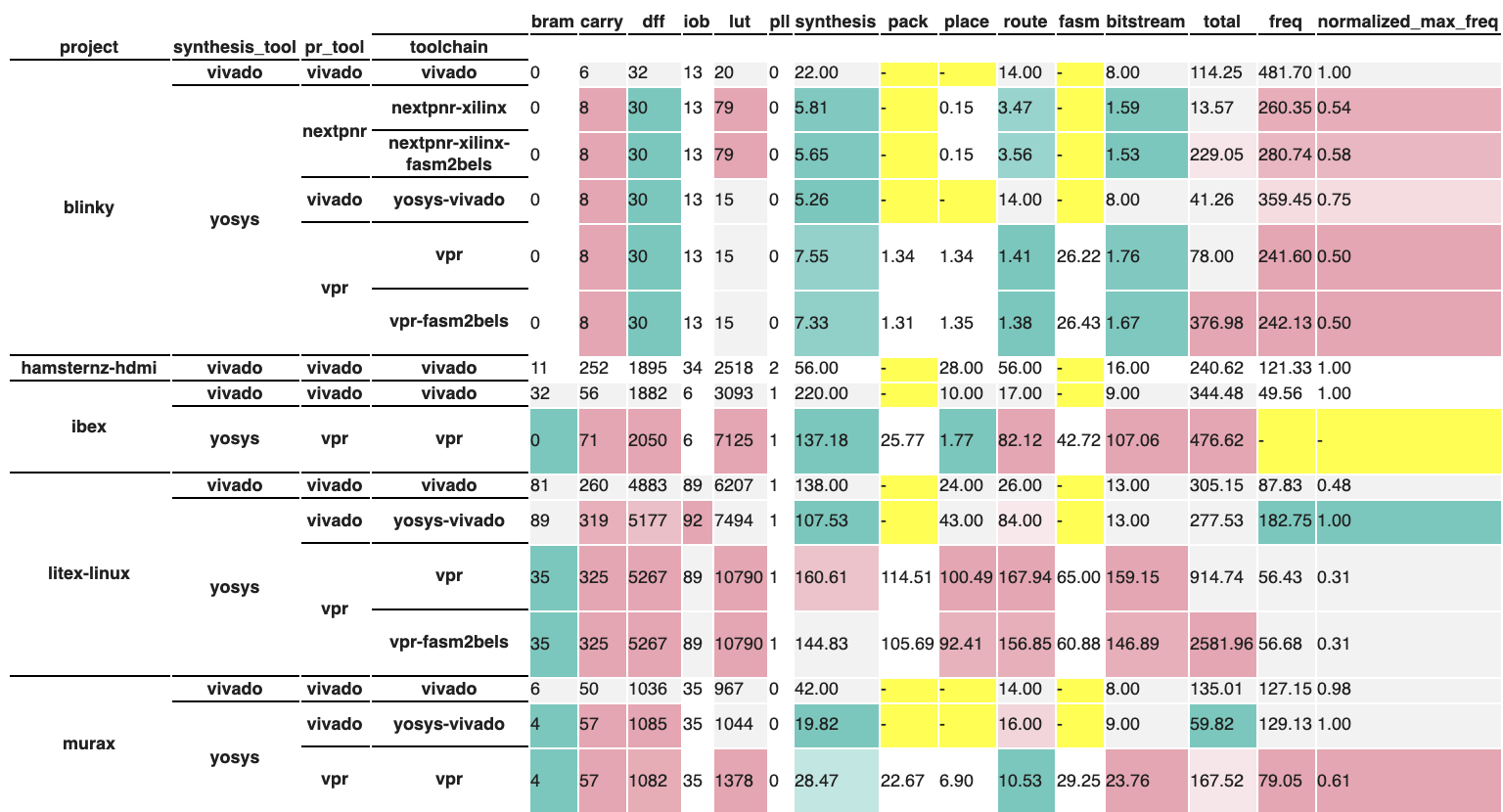
Then, we use the Visualizers in FTPVL to generate an IPython-compatible visualization that can be displayed.

vis = SingleTableVisualizer(
    eval1,
    styled_eval,
    version_info=True,
    custom_styles=custom_styles
)
display(vis.get_visualization())